Angular Momentum in Statistical Decay of Hot Nuclei

Laboratoire de Physique Fondamentale, FRANCE
1 July 1995
A statistical model for sequential binary decay of hot nuclei, treating the angular momentum consistently, and thus providing realistic angular distribution even in the case of intermediate mass fragment production, is described. An example of calculation is then given, and the weaknesses and applications of the model are discussed.
Latest version: http://phy.clmasse.com/angular.html
In intermediate energy heavy ion collisions, hot nuclei take birth with temperatures mostly lying under 5 MeV, but always with a sizeable spin, that is an unavoidable consequence of any mode of production. Statistical models, able to describe the decay of nuclei up to the highest excitations, exist, but until now, only for zero initial angular momenta [1]. Indeed, a large number of intermediate mass fragments are emitted, making the problem very difficult. So, finite spins were seldom considered, and only in case of sequential binary decay — which is a not so bad approximation given the relatively moderate temperature — and saddle point (or ridge line) transition state formalism [2] — which in contrary do not allow a consistent treatment of the angular momentum because of the too wide use of the rigid rotation condition. The calculation of the angular distribution was done as well with saddle point [3] as scission point [4] conditions, but independently of the other, beforehand fixed variables, the probability laws of which can thus not be reached.
In order to get a complete description, the best way is to choose the scission point, which is better suited, on one hand, to high excitation energies and angular momenta from the point of view of realistic reproduction of angular distributions [5] and account of the full phase space, and on the other hand, to natural reduction to Weisskopf’s standard formalism in case of light particle emission. The third, and actually strongest reason, is that it is the only one permitting the consistent introduction of angular momentum at all. In the present work, this is achieved similarly as in the extended Hauser-Feshbach model [6], but with much less computational requirement, so as to be suitable to event generation.
As in cellular division, the whole disintegration chain will thus be decomposed into sequential steps, each consisting of the splitting of a nucleus into two fragments that can be of any mass, charge, spin, and excitation energy provided they should satisfy the conservation laws. Sequential means the steps are totally unconnected, specifically in terms of Coulomb interaction, as if they were occurring far away from each other. Two main approximations have to be done: the sharp cut-off one will be taken for the transmission coefficients, and the angular momenta will be dealt with classically [3]. Weisskopf’s conventional formula [7], derived from Fermi’s golden rule and balance principle, will then take the simple form: $${d^4P\over dt~dE~d\vec n}={1\over2\pi\hbar}\intop_{\ell\lt\ell_{gr}}d\vec\ell~\delta(\vec\ell\cdot\vec n) {\omega_f(E^*-E, \vec I_0-\vec\ell) \over\omega_0(E^\times,\vec I_0)}\tag1.$$ It gives the transition rate $P$ for initial excitation energy $E^*$ and spin $\vec I_0,$ and final relative kinetic energy \(E\) and emission direction $\vec n,$ $\omega_0$ and $\omega_f$ being the respective state densities, and $\ell_{gr}=\sqrt{2\mu R^2(E-B)}/\hbar$ the grazing angular momentum for the inverse process, expressed as a function of the radius $R$ and height $B$ of the fission barrier, and of the reduced mass $\mu.$ Finally, $E^*=E^\times-Q,$ where $Q$ is the mass balance.
The state density $\omega_f$ is now written symmetrically between the fragments [8], namely as the folding of the individual densities, giving: $$\DeclareMathOperator{\Step}{\Theta}\omega_f(\varepsilon,\vec I)=\intop_0^\varepsilon d\varepsilon_1\int d\vec I_1~\omega_1(\epsilon_1,\vec I_1)\omega_2(\varepsilon-\varepsilon_1,\vec I-\vec I_1)\tag2.$$ The angular momentum is thus introduced and angular distributions available if a spin dependent parametrization is substituted for $\omega$ [9], adapted to the classical angular momenta [10] is taken: $$\omega(\varepsilon,\vec I)={\sqrt\pi\over12}{\exp\{2\sqrt{a\varepsilon}-I^2/2\sigma^2\}\over a^{1/4}\varepsilon^{5/4}(2\pi\sigma^2)^{3/2}}\tag3.$$ Here, $a$ is the level density parameter and $$\sigma^2=0.0888\sqrt{a\varepsilon}A^{2/3}/\hbar^2\equiv J\sqrt{\varepsilon/a}/\hbar^2\tag4,$$ $J$ being the effective moment of inertia for a nucleus of mass number $A.$
Now, all these formulae are put into (1), which is then integrated over $E$ and $\vec n,$ yielding: $$\begin{multline} \hspace2em{dP\over dt}\propto\intop_B^{E^*}dE\intop_0^{E^*-E}d\varepsilon_1{\exp\{2\sqrt{a_1\varepsilon_1}+2\sqrt{a_2\varepsilon_2}\}\over(\varepsilon_2\varepsilon_2)^{5/4}(\sigma_1\sigma_2)^3}\times\\ \intop_{\ell\lt\ell_{gr}}{d\vec\ell\over\ell}\int d\vec I_1 \exp\left\{-{I_1^2\over2\sigma_1^2}-{I_2^2\over2\sigma_2^2}\right\}\hspace2em\tag5 \end{multline}$$ with the short hands: $\varepsilon_2=E^*-E-\varepsilon_1,$ $\vec I_2=\vec I_0-\vec I_1-\vec\ell,$ each of the indexes $1$ and $2$ referring to one of the fragments. For the light particles, until the α one, that are emitted in their ground state, $\omega$ is replaced by $\delta(\varepsilon)\delta^3(\vec I),$ and the usual equation is found again. In (5), all the information on the probability densities of the final observables is contained, and available by partial differentiation.
The integration has been performed by a Monte Carlo procedure. To get a rough expression of the relative likelihood of mass and charge, some further approximations have been done, in particular the use of the constant values: $a_1(E^*-E)/(a_1+a_2)\equiv a_1T^2$ (thermal equilibrium), $B+\ell^2/2\mu R^2=E^*-(a_1+a_2)T^2$ (most probable value) and $\vec L=\mu R^2\vec I_0/(J_1+J_2+\mu R^2)$ (rigid rotation condition) instead of, respectively $\varepsilon_2,$ $E,$ and $\vec n$ only where necessary and where their variations could be neglected. This leads to: $$\begin{multline} \hspace2em{dP\over dt}\propto{a\over\sqrt{(a_1a_2)^3JT^5}} \exp\left\{2\sqrt{a\left(E^*-B-{\hbar^2I_0^2\over2(J+\mu R^2)}\right)}\right\}\times\\ {2JrT\over\hbar I_0}\intop_0^{\sqrt{{r\over2JT}}}dx~e^{-x^2}\hspace2em\tag6, \end{multline}$$ where $J=J_1+J_2,$ $a = a_1+a_2,$ and $r=\mu R^2/(J+\mu R^2).$ The so introduced errors have afterward been largely compensated by rejection techniques. The other conditional probability densities are listed below ($\Step$ is the step function): $$\begin{multline} \hspace2em f(\vec\ell)\propto{1\over\ell} \exp\left\{-{\hbar^2(\vec I_0-\vec\ell)^2\over2JT}+2\sqrt{a\left(E^*-B-{\hbar^2\ell^2\over2\mu R^2}\right)}\right\}\times\\ \Step\left(E^*-B-{\hbar^2\ell^2\over2\mu R^2}\right)\hspace2em\tag7, \end{multline}$$ $$\begin{multline} \hspace2em f(E|\vec\ell)\propto\int_0^{E^*-E}d\varepsilon {\exp\{2\sqrt{a_1\varepsilon}+2\sqrt{a_2(E^*-E-\varepsilon)}\}\over[\varepsilon(E^*-E-\varepsilon)]^{5/4}}\times\\ \Step\left(E-B-{\hbar^2\ell^2\over2\mu R^2}\right)\Step(E^*-E)\hspace2em\tag8, \end{multline}$$ $$f(\varepsilon_1|E)\propto{\exp\{2\sqrt{a_1\varepsilon_1}+2\sqrt{a_2(E^*-E-\varepsilon_1)}\}\over[\varepsilon_1(E^*-E-\varepsilon_1)]^{5/4}} \Step(\varepsilon_1)\Step(E^*-E-\varepsilon_1)\tag9,$$ $$f(\vec I_1|\vec\ell)\propto\exp\left\{-{I_1^2\over2\sigma_1^2}-{I_2^2\over2\sigma_2^2}\right\} \Step\left(E^*-B-{\hbar^2\ell^2\over2\mu R^2}-{I_1^2\over2\sigma_1^2}-{I_2^2\over2\sigma_2^2}\right)\tag{10}.$$ The emission direction is simply uniform and perpendicular to $\vec I,$ and the velocities are deduced from $E$ and the masses, of course taking the recoil into account so that the initial conditions of the next step are fully defined. Each product fragment is proceeded with in the same way until they all are particle stable.
On input, a sample of nuclei with fixed or complying with a probabilistic law masses, charges, excitation energies, and spins must be provided, for instance by the first phase of an event generator. The output consists of an event with statistical weight 1, wholly specified by determinate values of the masses, charges, and velocities of all the emitted particles.
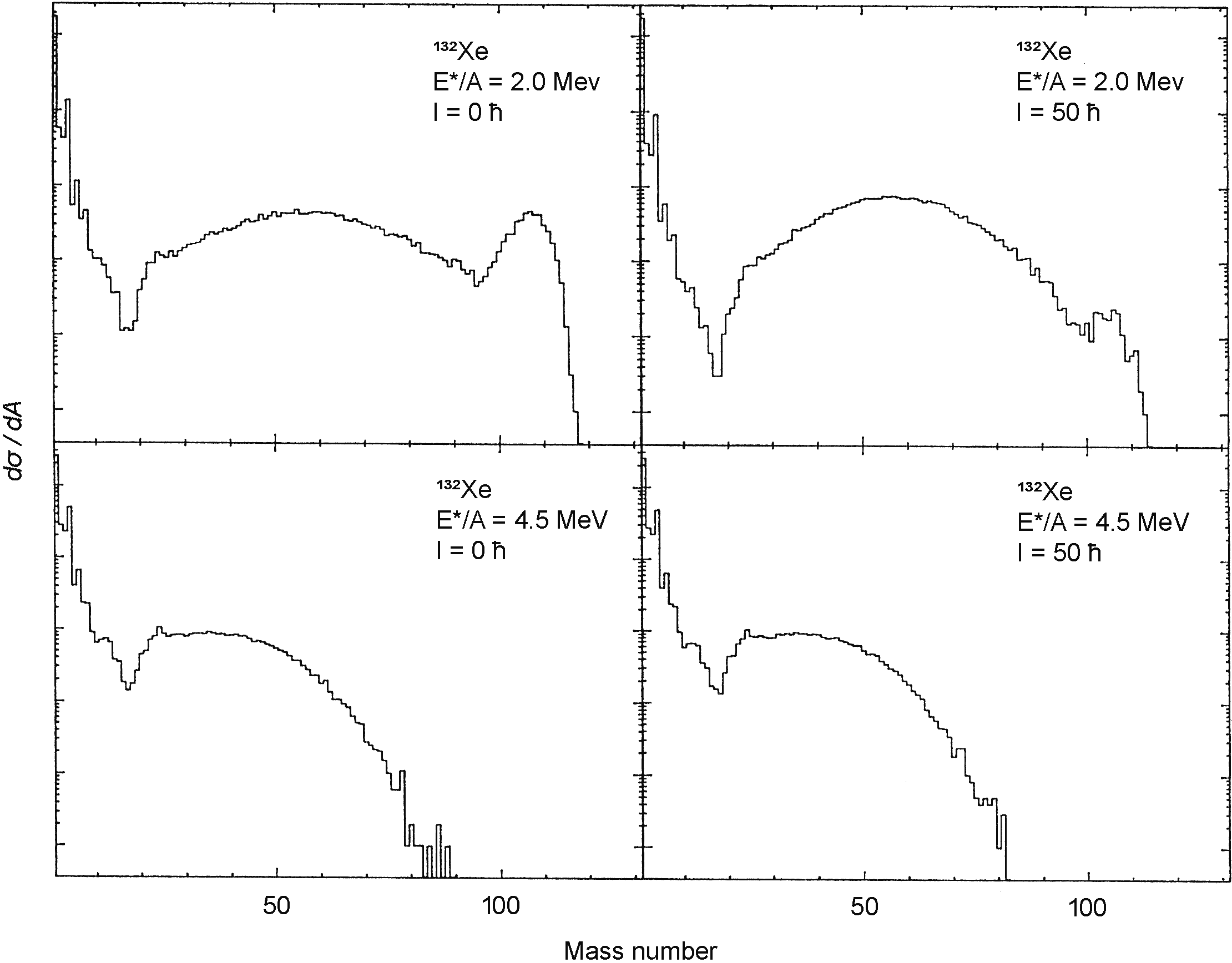
Figure 1 depicts an example of calculation for several initial excitation energies and spins with realistic level density parameters, masses, and barrier heights, and show the action of the spin on the mass distribution. The most striking feature, besides the softening of the slope, is the partial disappearance of the evaporation residue component in benefit of the fission one.
At this point, it must be recalled a lowering of fission likelihoods for increasing apparent temperature would occur experimentally. In fact, fission takes place at the end of the desexcitation process. When the temperature gets higher and higher, the nucleus would then become too light to undergo a final scission. This can be described in terms of a Fokker-Planck equation [11], by which a transient time is required for the nucleus to reach the saddle point, but with the time scale of evaporation getting smaller and smaller. In principle, such an effect could be roughly accounted for, but this was not done for several reasons. First, for a nucleus emerging from a collision, the initial shape is difficult to define, and is surely not spherical. Then, an excited cluster change its mass continually, possibly very quickly, and an origin for the time is hard to determinate. More generally, the appearance of a transient time is a non-equilibrium phenomenon, and is hence incompatible with the statistical equilibrium hypothesis. Its consistent treatment is therefore far beyond the scope of this relatively simple model.
In summary, a complete simulation of the statistical mechanics of the sequential binary decay of a hot and spinning nucleus is obtained, giving reliable results in all possible conditions, except at a too high or too low temperature. Contrary to most of the preceding models, the full equation, including angular momentum dependence, is worked out, the only physical approximations being the sharp cut-off for the transmission coefficients and the classical treatment for the angular momenta.